AdvancedTraining_11_Compact_Models.pdf
Compact Models,Advanced Resistances
Compact Representation
of Heat Sinks
-Why Compact Representation in System Level Model?
– Faster Solution
– Less Grid
– Fewer Iterations - Simplified Conjugate Heat Transfer Problem
– Much Easier to Work With and Debug Compact Representation of Heat Sinks
-Attributes of a Good Heat Sink Compact Model:
– Preserve the Flow Characteristics Through and Around the Heat Sink
– Correct Pressure Drop (Contraction, Expansion, Friction)
– Correct Bypass to Sides and Top
– Preserve the Conduction Characteristics in the Heat Sink Base and Fins (Heat Sink Efficiency)
– Preserve the Convection Effects of the Base and Fins. (Forced or Natural Convection)
- The Heat Sink SP Compact Model Provides a Good representation of these attributes and saves modeling and solve time for System Level Modeling
-The Pressure Drop Terms Include:
– Sudden Contraction Entrance Collapsed Resistance.
– Sudden Expansion Collapsed Resistance for Exit and Top.
– Volume Resistance for the Laminar or Turbulent Frictional Flow in the Heat Sink Channels
- Heat Transfer is Treated Using a Volumetric Based Heat Transfer Coefficient. This Coefficient is a Function of Flow Rate for Turbulent Flow and Constant for Laminar.
- The Heat Transfer Model Does Not Account For Fin Efficiency. Under Predicts Base Temperature for Highly Convective Cases Where Fins Are Thin.
Compact Representation of
Heat Sinks
- Option 2: Approximation Based on Computational or Physical Wind Tunnel Characterization
– Represent Heat Sink Base As a Conducting Cuboid
– Perform(Separate) Computational/Physical Wind Tunnel Analysis to Determine Flow Impedance Characteristics of Fins
– Account for Impedance of Heat Sink Fins With Volume Resistance in System Level Model
– Account for Heat Dissipation of Fins with Volume Heat Transfer Coefficient in System Level Model
Resistance and
-Option 2: Approximation Based on Computational Wind Tunnel Characterization (Cont.)
– Duct Detailed Fins (Only) of Heat Sink With Computational Domain: Use Symmetry Faces on 4 Long Sides and Open Faces on Ends
– Extend the Computational Domain as Shown
– Use Fixed Flow Device and Collapsed Resistance (or Nothing) for Ends
Wind Tunnel Characterization (Cont.)
– Use ΔP vs. V Data to Define Equivalent Non-Collapsed Resistance
– Can Use Advanced Resistance Attribute (When ΔP Is Not α V2
– Refer to Resistance Calculation Slides Later in this Lecture)
– Typically Use Standard Resistance Attribute (Iteratively If ΔP Is Not α V2)
– Replace Detailed Fins (Cuboids) With Non-Collapsed Resistance
– Re-Run One Case to Ensure that Computed ΔP’s for Detailed and Compact Models Agree
Modeling Grilles, Filters and
Other Flow Resistances
- Use a (Collapsed or Non-Collapsed) Resistance With Appropriate
Loss Coefficient
- Recall, Definition of Loss Coefficient
Δp = f (ρv2/2) (Collapsed)
Δp/Δx = fx (ρv2/2) (Non-Collapsed)
Δp/Δy = fy (ρv2/2) (Non-Collapsed)
Δp/Δz = fz (ρv2/2) (Non-Collapsed)
where:
v = velocity (device or approach)
f = loss coefficient
Modeling Flow Resistances
- Available Loss Coefficient Options
– Standard
– Assumes Δp α v2
– Constant Loss Coefficient f
– Advanced
– Allows complicated Δp dependence on v
– Loss Coefficient f not Constant
f = a/Re + b/Reα
in which,
f = loss factor (as before)
Re = ρUL/μ = Reynolds No. based on
a user specified length scale
a,b,α = constants specified by the user
Modeling Flow Resistances
- Where Do I Get Loss Coefficients?
– Reference Texts, e.g., Fried and Idelchick
– Manufacturer Data
– Perform Computational Wind Tunnel Analysis on Device
- Advice on Loss Coefficients
– Use Standard Model If You Have ΔP~V2
– Most Turbulent, High Re Flows
– Use Advanced Model If You Have ΔP~V, ΔP~V1.7, etc.
– Laminar and Transitional, Lower Re Flows
– Can Always Use Standard Model If You’re Willing to Iterate
Example: Given ΔP=kV
-This Case is Typical for Laminar Flow
- If Resistance Can Be Modeled As “Thin”:
– Resistance Type: Planar
– Loss Coefficients Based On: Approach Velocity
– Resistance Formula: Advanced
– Length Scale (L): 1 m
– A Coefficient: (2 L k)/μ
– B Coefficient: 0
– Index: 0
Other Compact Models
The Flow Losses and Heat Addition of All Components/Modules in the Analysis Need to be Accounted For.
- In Cases Where the Details of those Components Are Not Important, the Above is Still True.
- Create Compact Models for These:
– Guess the Losses and Heat (Typically Early in Concept Design and Optimization)
– Use a Combination of Collapsed or Volumetric Resistances With Associated Sources.
– Create Detailed Windtunnel Models of Modules, Characterize for Losses and Create Good Compact Models. (Later when more information is available).
– This Process is Similar to the Manual Heat Sink Compact Model
Angled Resistances
-There are 2 Ways to Create this Angled
Resistance In Flotherm.
– Use flotherm.com and go to the User Support Center. Choose [Support], Then [Web Parts].
– Do it Yourself Using the Instructions on the Following Page.
標簽: 點擊: 評論: